Using a Deep Neural Network to Play Flappy Bird via Reinforcement Learning
Introduction to Reinforcement Learning
Reinforcement learning differs from classical machine learning methods such as supervised and unsupervised learning. A supervised learning algorithm expects training data, containing inputs and their corresponding outputs. Algorithms will be applied to create a mapping between these input and outputs so that when given a previously unseen input it will to the best of its ability predict the correct output.
Unsupervised learning, on the other hand, aims to find patterns from sets of data, no output data is given. The algorithm chosen is expected to find the hidden structures in the data.¹ ²
Reinforcement learning differs from both of these as it has no initial datasets to work with. An agent takes actions within a given environment. When an action is taken, feedback is given in the form of a reward. The better the action the better the reward. In the reinforcement learning algorithm, the agent will be in a state at any given time. The agent will then take an action in its state and be given a reward. The agent learns from these rewards to take better actions in the future. The end goal is to have an agent take the best step in a given state (I.e. the step that maximises the reward).
We officially define these terms below ³ ⁴:
- Agent: The decision maker and learner, observes the environment and takes actions
- State: Current situation of the agent in the environment.
- Environment: The world in which the agent decides on actions and learns from the actions
- Reward: The feedback given from the environment when an action is taken

If we take Pac-Man as an example. The agent, environment, states and reward would be as followed ⁵:
- Agent: the “PacMan” itself.
- Environment: The grid in which the “PacMan” moves
- Reward: The “PacMan” will receive a positive reward if it eats food and a negative reward if a ghost catches it.
- State: This could consist of the current position of the “PacMan”, the current position of the ghosts and the positions of the points.
Armed with this knowledge, we aim to use reinforcement learning to train an agent to learn Flappybird.

In this case, we have:
- Agent: The Bird
- State: A vector consisting of the current position of the bird, its velocity and the distances and positions of the next 2 pipes to the bird.
- Reward: The further the bird progresses through the course before crashing, the greater the reward
- Environment: The game in which the bird takes actions
As well will have 2 possible actions, move up, or take no action.
Key Concepts and Algorithms Used
We solve the reinforcement learning problem using a Deep-Q Network. This is a common solution to reinforcement learning problems. To understand where these networks originate from we first must understand Markov Decision Processes (MDPs).
MDPs
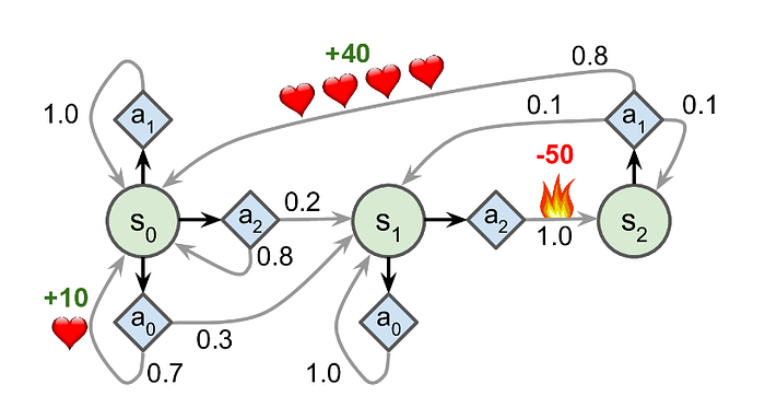
Markov Decision Processes (MDPs) are probabilistic state models containing a state space, initial state, actions for each state, transition probabilities, rewards and a discount factor. They can visually show all the possible states for an agent, the probabilities of moving to states after taking an action and the rewards that occur when actions are taken. There are no goal states, the agent receives a reward based on the action taken in a given state¹².
For example, in this MDP, if the agent starts in state S0, it can take action A2 and end up in state S1 with a 20% probability or stay in state S0 with an 80% probability. If for example, it is in state S2 after taking action A1 it has an 80% probability of getting a +40 reward and moving back to state S0.
State Values
The optimal state value (V*(s)) of a state is defined as the sum of all discounted future rewards the agent can expect on average after reaching a state s, assuming it acts optimally (taking the action with the highest reward over an infinite horizon¹³) ¹⁴ (p627). The equation for V*(s) is below.

We first calculate the expected reward for each action. This is the sum of the reward for all states resulting from that action plus the discounted future reward of those states (V*(s’)). We multiply this combined reward by the probability of moving into that state.
From this equation, we can create an algorithm to work out the optimal state value for each state. We initialise all state values to 0 and then run the following algorithm):
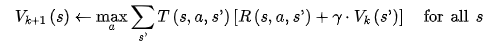
For each iteration k the equation is run for every state s ¹⁵.
Q-Values
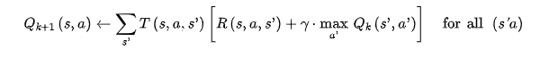
After calculating the optimal state values, we must then formulate an optimal policy for the agent. This can be achieved by using Q-values. Which are optimal state-action values. These are defined as the sum of discounted future rewards the agent can expect (assuming it acts optimally) on average after it reaches state s and chooses action a ¹⁴ (p628).
We can calculate Q values using the following iteration algorithm. The initial Q values are set to 0 and for each iteration k the equation is run for every state s action pair (s, a).¹⁶
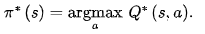
The optimal policy in each state is then defined as the action that maximises the possible Q values. Since if we maximise the Q value, we maximise the future rewards of the agent ¹⁴ (p628).
Q-Learning Algorithm
We must then consider that initially, we do not have an idea of the transition probabilities and the resulting rewards that arise from those transitions. It must experience the states and the transitions to compute the rewards and it must experience this multiple times to compute an estimate of the transition probabilities¹⁴ (p629).
The Q-learning algorithm is an adaptation of the Q-value function where we assume no knowledge of the transition probabilities and the rewards. We watch an agent play and continually improve estimates of Q values. Once we have Q values we can choose the action that has the maximal Q value¹⁴ (p630).
This algorithm can be seen below:
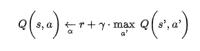
For this algorithm, we set the initial Q values to 0 and run the algorithm. We can introduce learning rate decay as well¹⁴ (p631).
Deep Q Networks
The main issue arises when we start to scale the MDP. For each state, action pair we must have an estimate of the Q value. So as the number of states and actions increases, so does the number of estimates we must keep track of .¹⁴ (p633)
To solve this issue we can use a Deep Q network. Whereby we find a function to estimate the Q value based on any given state and action. That function is the output of a Deep Neural Network, which is appropriately titled a Deep Q Network¹⁴ (p633).
Based on Bellman, the approximate Q value computed by the network should be as close to the reward we get plus the discounted value of playing optimally from there on (I.e. the maximal Q value for a given state over all the actions). To find this value, we execute the DQN on the next state for all possible actions. We take the maximal Q value from the outputs, as we assume that we are playing optimally. Then we can discount it and add the current reward to it. This provides us with the target Q value¹⁴ (p633–634).
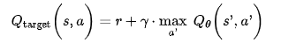
When training the network, we compute a predicted Q value using the deep Q network and then calculate this target Q value. We aim to minimise the squared error between these 2 values and train the network as expected¹⁴ (p634).
Based on the Deep Q Network, there are a couple of variant networks that improve performance.
Using 2 Networks
Currently, the model is used to make predictions and to set its own targets. I.e. it outputs both the Q values it should be achieving and the Q values it is currently predicting. This can create a feedback loop and make the network unstable. Instead, we have 2 models, one to output the predicted Q values, which then becomes the one we use when selecting actions and one to output the target Q values¹⁴ (p639).
This target model is simply a clone of the prediction model, we copy the parameters from the prediction model into the target model at fixed intervals¹⁴ (p639).
Dueling Deep Q Networks
First note that we can express the Q value of a state action pair as seen below, where V(s) is the value of the state and A(s,a) is the advantage of taking action a in state s, compared to all other actions. The value of the state V(s) is equal to the Q value of the best action (a*) for that state as we are assuming that we will act optimally. Therefore Q(s, a*) = V(s) and we can imply that the A(s, a*) = 0. ¹⁴ (p641)
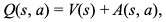
With a duelling Q network, we estimate the advantage of each action and the value of the state. As seen above, the best action should have an advantage of 0. We subtract the maximum predicted advantage from all advantages and then add these to the state value to generate Q values for each action. Therefore, for a given state, the action with the largest advantage will be the best action and will provide us with the largest Q value¹⁴ (p641).
Methodology
Environment
To set up our environment, we use the PyGame Learning Environment⁶. This is a library giving access to many games that can be used in a reinforcement learning manner. Using this means that we do not have to set up our environment. We simply feed the actions to an instance of the Flappybird module in this package, and it will return the reward and state.
The environment can be instantiated as so, here we show the list of possible actions and the current state of the agent in the environment.
game = FlappyBird(width=256, height=256)
p = PLE(game, display_screen=False)
p.init()
actions = p.getActionSet()
action_dict = {0: actions[1], 1: actions[0]}
state = p.getGameState()
Network
For the network, we opt for a simple dynamic neural network. In this way, the network can either operate as a Q network or a duelling Q network. The input is the current state, the output is a vector of Q values for each possible action. We have 4 hidden layers, increasing the number of neurons as the network progresses, applying a ReLU6 activation after each layer.
class DQN(torch.nn.Module):
    def __init__(self, input_dim, output_dim, network_type='DDQN', *args, **kwargs) -> None:
        super().__init__(*args, **kwargs)
        self.input_dim = input_dim
        self.output_dim = output_dim
        self.network_type = network_type
        self.layer1 = nn.Linear(input_dim,64)
        self.layer2 = nn.Linear(64, 128)
        self.layer3 = nn.Linear(128, 256)
        self.layer4 = nn.Linear(256, 512)
        self.layer5 = nn.Linear(512, 512)
...
    def forward(self, x):
        x = F.relu6(self.layer1(x))
        x = F.relu6(self.layer2(x))
        x = F.relu6(self.layer3(x))
        x = F.relu6(self.layer4(x))
        x = F.relu6(self.layer5(x))
Additionally, we chose to have a different network created based on the arguments. We can easily create a duelling variant of the DDQN by having 2 output layers to compute the state and advantage values. These are then combined to produce the output.
class DQN(torch.nn.Module):
    def __init__(self, input_dim, output_dim, network_type='DQN', *args, **kwargs) -> None:
        super().__init__(*args, **kwargs)
    ...
        if network_type == 'DuelingDQN':
            self.state_values = nn.Linear(512,1)
            self.advantages = nn.Linear(512, output_dim)
        else:
            self.output = nn.Linear(512, output_dim)
    ...
    def forward(self, x):
    ...
        if self.network_type == 'DuelingDQN':
            state_values = self.state_values(x)
            advantages = self.advantages(x)
            output = state_values + (advantages - torch.max((advantages), dim=1, keepdim=True)[0])
            return output
        else:
            return self.output(x)
Cache Recall
We will require a memory system to store our experiences so that we can randomly sample a batch of experiences to learn from. We create a simple class based on the double-ended queue Python structure. We add functions for appending data to the queue and randomly sampling a batch of data. These functions will be used later by our agent to store the experiences as it moves through the environment and to sample a batch of these experiences to train the policy network.
class MemoryRecall():
    def __init__(self, memory_size) -> None:
        self.memory_size=memory_size
        self.memory = deque(maxlen = self.memory_size)

    def cache(self, data):
        self.memory.append(data)

    def recall(self, batch_size):
        return random.sample(self.memory, batch_size)

    def __len__(self):
        return len(self.memory)
Agent
To create the action we require the following functions:
- Function to choose an action
- Function to compute the Q values, loss and optimisation of the models
- The main training function that should process the agent as it moves through states and takes action
Choosing an Action
Choosing an action is fairly simple, we follow an epsilon-greedy policy⁷. In this policy, the agent chooses a random action with probability ε and a greedy action with probability (1-ε). A greedy action is one that maximises the Q value, since if we maximise the Q value we maximise the future rewards that the agent will incur. Since the policy network outputs the approximate Q value for each possible action, we simply chose the action that has the largest output from the network.
@torch.no_grad()
def take_action(self, state):
    self.eps = self.eps*self.EPS_DECAY_VALUE
    self.eps = max(self.eps, self.EPS_END)
    if self.eps < np.random.rand():
        state = state[None, :]
        action_idx = torch.argmax(self.policy_net(state), dim=1).item()
    else:
        action_idx = random.randint(0, self.action_dim-1)
    self.steps_done += 1
    return action_idx
One key element of the epsilon-greedy policy is the decay of our hyperparameter ε. We initially want this parameter to be 1.0, and then slowly decayed over time. This is to ensure that the agent explores the possible states and transitions to build up a diverse list of experiences rather than just those states that lead to the maximal rewards. If the agent just chose the optimal action based on the reward, it may lead to sub-optimal performance as it is not choosing to transition into states that could lead to even greater rewards in the future. We also want the agent to be exploiting the states of the environment that lead to better rewards. Hence, the epsilon-greedy policy is chosen.
As the agent progresses, we decay the epsilon value. This is because, at the start of the training process, the agent has not yet explored the environment nor has the network been trained. Therefore, we want to fill up the experience buffer with diverse experiences. However, as more experiences are encountered, we want the agent to exploit the actions that give the largest reward as we are more confident that it has explored the state space adequately ⁸ ⁹.
Training the model
We implement the following function for training.
def optimize_model(self):
    if len(self.cache_recall) < self.BATCH_SIZE:
        return
    batch = self.cache_recall.recall(self.BATCH_SIZE)
    batch = [*zip(*batch)]
    state = torch.stack(batch[0])
    non_final_mask = torch.tensor(tuple(map(lambda s: s is not None, batch[1])), device=self.device, dtype=torch.bool)
    non_final_next_states = torch.stack([s for s in batch[1] if s is not None])
    action = torch.stack(batch[2])
    reward = torch.cat(batch[3])
    next_state_action_values = torch.zeros(self.BATCH_SIZE, dtype=torch.float32, device=self.device)
    state_action_values = self.policy_net(state).gather(1, action)
    with torch.no_grad():
        next_state_action_values[non_final_mask] = self.target_net(non_final_next_states).max(1)[0]
    expected_state_action_values = (next_state_action_values * self.GAMMA) + reward
    loss_fn = torch.nn.SmoothL1Loss()
    loss = loss_fn(state_action_values, expected_state_action_values.unsqueeze(1))
    self.optimizer.zero_grad()
    loss.backward()
    self.optimizer.step()
First, we sample a batch of data and reform the batch so that we can easily retrieve the states, actions, rewards and next states. We then collect the data as followed.
batch = self.cache_recall.recall(self.BATCH_SIZE)
batch = [*zip(*batch)]
state = torch.stack(batch[0])
action = torch.stack(batch[2])
reward = torch.cat(batch[3])
We must consider that some of the next states, as a result of taking the action will be None as the Bird will have collided with a pipe. Therefore, we create a mask to filter out the next states that are not None. As well we also collect the next states that are not None.
non_final_mask = torch.tensor(tuple(map(lambda s: s is not None, batch[1])), device=self.device, dtype=torch.bool)
non_final_next_states = torch.stack([s for s in batch[1] if s is not None])
As per the theory, we pass the state through the policy network in order to compute an estimate of the Q values for each state-action pair. As the network outputs a Q value for every action for a given state, we must only collect those Q values for the action taken.
state_action_values = self.policy_net(state).gather(1, action)Then we compute the expected Q values. This is done by taking the output of the target network for each next state and then taking the maximum, making sure that we filter out the next states that have a None value (as these datatypes cannot be processed by the network). We then multiply this as per the equation to retrieve our expected Q values.
with torch.no_grad():
    next_state_action_values[non_final_mask] = self.target_net(non_final_next_states).max(1)[0]
expected_state_action_values = (next_state_action_values * self.GAMMA) + reward
To train the network, we compute the L1 loss between the estimated Q values from the policy network and the expected Q values from the target network. We then run the needed steps to train the policy network.
loss_fn = torch.nn.SmoothL1Loss()
loss = loss_fn(state_action_values, expected_state_action_values.unsqueeze(1))
self.optimizer.zero_grad()
loss.backward()
self.optimizer.step()
Main training function
Lastly, we create the main processing function for the agent. We run the agent for a set number of episodes. Here we define an episode as a single gameplay. The Bird will take a sequence of actions until it crashes into a pipe.
The code for this portion of the agent is fairly self-explanatory. We reset the game each episode, taking the initial state. Then as the agent takes a new action, we store the reward, action, state and next state (state moved into as a result of taking the action) in our cache memory. We then train the model and update the target network.
def train(self, episodes, env):
    self.steps_done = 0
    for episode in range(episodes):
        env.reset_game()
        state = env.getGameState()
        state = torch.tensor(list(state.values()), dtype=torch.float32, device=self.device)
        for c in count():
            action = self.take_action(state)
            reward = env.act(self.action_dict[action])
            reward = torch.tensor([reward], device=self.device)
            action = torch.tensor([action], device=self.device)
            next_state = env.getGameState()
            next_state = torch.tensor(list(next_state.values()), dtype=torch.float32, device=self.device)
            done = env.game_over()
            if done:
                next_state = None
            self.cache_recall.cache((state, next_state, action, reward, done))
            state = next_state
            self.optimize_model()
            self.update_target_network()
...
The target network is updated in the following function. Instead of simply copying the policy network parameters to the target network, we use a soft update¹⁰. In this case, Tau is set to 0.005, therefore when the target network is updated it will combine 0.5% of the policy network parameters with 99.5% of the target network parameters.
def update_target_network(self):
    target_net_state_dict = self.target_net.state_dict()
    policy_net_state_dict = self.policy_net.state_dict()
    for key in policy_net_state_dict:
        target_net_state_dict[key] = policy_net_state_dict[key]*self.TAU + target_net_state_dict[key]*(1-self.TAU)
        self.target_net.load_state_dict(target_net_state_dict)
Lastly, if the episode has ended we plot the data and store the networks.
...
if done:
    self.episode_durations.append(c+1)
    self.plot_durations()
    print("EPS: {}".format(self.eps))
    print("Durations: {}".format(c+1))
    print("Score: {}".format(env.score()))
    torch.save(self.target_net.state_dict(), self.network_type+'_target_net.pt')
    torch.save(self.policy_net.state_dict(), self.network_type+'_policy_net.pt')
    break
Results
For our main run, we used a duelling deep Q network and ran this for just over 12000 episodes. We kept the epsilon decay quite light, to make sure that the agent had adequate time to explore.
We can see from the training graph that the agent learns to traverse the environment very well, being able to run for thousands of actions without crashing into a pipe.
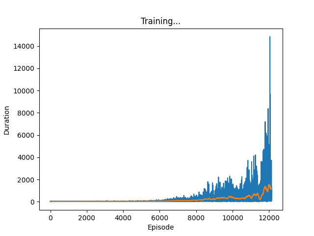
The following animation highlights this trained agent in action.

Full code is available on GitHub: https://github.com/nathanwbailey/flappy_bird_reinforcement_learning
[1]: Unsupervised learning, Wikipedia. https://en.wikipedia.org/wiki/Unsupervised_learning
[2]: Unsupervised learning, Geeks for Geeks. https://www.geeksforgeeks.org/supervised-unsupervised-learning/
[3]: Introduction to reinforcement learning for beginners. Analytics Vidhya. https://www.analyticsvidhya.com/blog/2021/02/introduction-to-reinforcement-learning-for-beginners/
[4]: Geron, A. (2019). Hands-On Machine Learning with Scikit-Learn, Keras and TensorFlow (2nd ed.). O’Reily Media. p610
[5]: Reinforcement Learning in Pacman, Gnanasekara, A http://cs229.stanford.edu/proj2017/final-reports/5241109.pdf
[6]: PLE: A Reinforcement Learning Environment, Read the Docs. https://pygame-learning-environment.readthedocs.io/en/latest/
[7]: Geron, A. (2019). Hands-On Machine Learning with Scikit-Learn, Keras and TensorFlow (2nd ed.). O’Reily Media. p632–634
[8]: Epsilon-Greedy Algorithm in Reinforcement Learning. Geeks for Geeks. https://www.geeksforgeeks.org/epsilon-greedy-algorithm-in-reinforcement-learning/
[9]: Strategies for Decaying Epsilon in Epsilon-Greedy. Medium. https://medium.com/@CalebMBowyer/strategies-for-decaying-epsilon-in-epsilon-greedy-9b500ad9171d
[10]: Continuous control with deep reinforcement learning. Timothy P. Lillicrap. https://arxiv.org/abs/1509.02971
[11]: FlappyBird, N64 Squid. https://n64squid.com/flappy-bird/
[12]: Reinforcement Learning 101, Towards Data Science. https://towardsdatascience.com/reinforcement-learning-101-e24b50e1d292
[13]: Markov Decision Processes, Gibberblot https://gibberblot.github.io/rl-notes/single-agent/MDPs.html
[14]: Hands-On Machine Learning with Scikit-Learn, Keras and Tensorflow. Aurelien Geron.
[15]: Value Iteration vs. Policy Iteration in Reinforcement Learning. https://www.baeldung.com/cs/ml-value-iteration-vs-policy-iteration
[16]: Bootcamp Summer 2020 Week 3 — Value Iteration and Q-learning https://core-robotics.gatech.edu/2021/01/19/bootcamp-summer-2020-week-3-value-iteration-and-q-learning/